Designing a 2D Transformer Core: Steady-State Simulation in ElmerFEM (Part 2)
In this second part of our series, we transition from geometry preparation in FreeCAD to the simulation environment of ElmerFEM. If you missed Part 1, you can catch up via the link.
ElmerGUI streamlines the workflow by managing the Solver Input File (.sif) directly through its interface. In this stage, we will compute the static magnetic flux generated by the transformer’s primary winding and later apply a load to the secondary winding to validate our Finite Element Method (FEM) results against analytical calculations.
Understanding ElmerGUI
Before we start, it is important to understand that ElmerGUI is a great tool for those starting with Elmer. However, you will soon find that the core configuration eventually leads back to the .sif file, which we will learn to edit in this post.
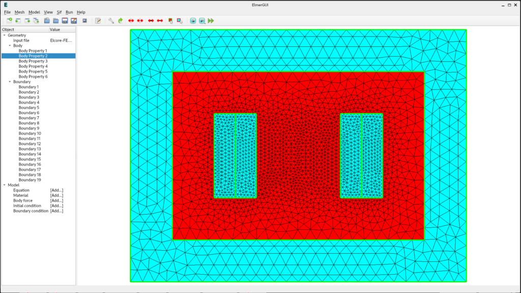
First Steps: Importing and Scaling
The first task is to import the mesh we generated previously. Go to File >> Open and select your .unv file.
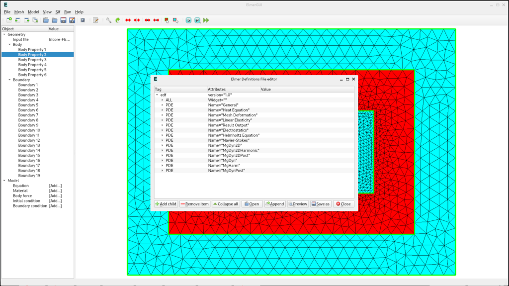
For the model to work correctly, we need two specific solvers that aren’t active by default in the UI:
- Go to File >> Definitions.
- Click the Append button.
- Navigate to the
edf-extrafolder and selectmagnetodynamics2d.xmlandmagnetodynamics.xml.
Important Note on Units: If you modeled your geometry in millimeters or inches, you must add a Coordinate Scaling factor. Go to Model >> Setup and set the scale to
0.001(to convert mm to meters), as Elmer operates in SI units.
Setting Up the Equation
We must inform Elmer what physics it needs to solve.
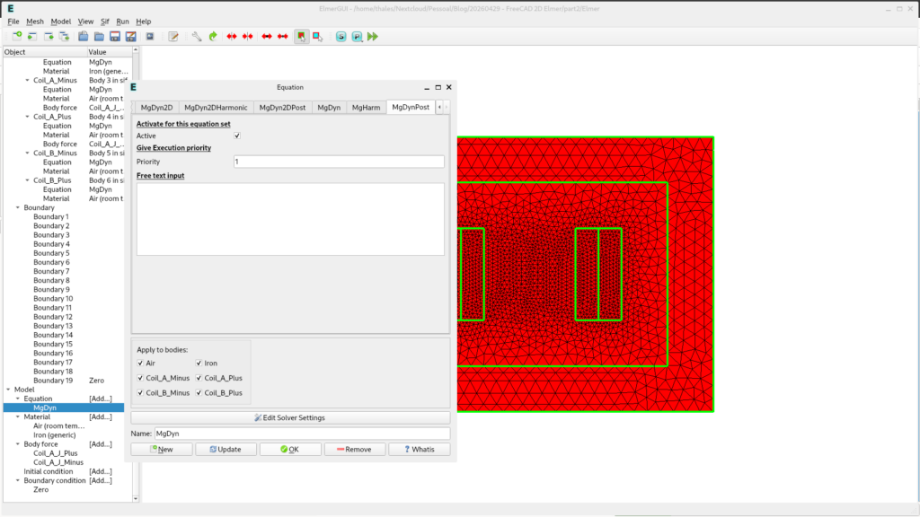
- In the left sidebar, under Model, click Equation >> Add.
- In the MgDyn2D tab, activate the solver and apply it to all bodies.
- Set the Priority to 2 (higher numbers indicate higher priority).

- Now look for MgDynPost (used for post-processing results). Activate it and set its Priority to 1.
- Name this set “MgDyn” before clicking OK.
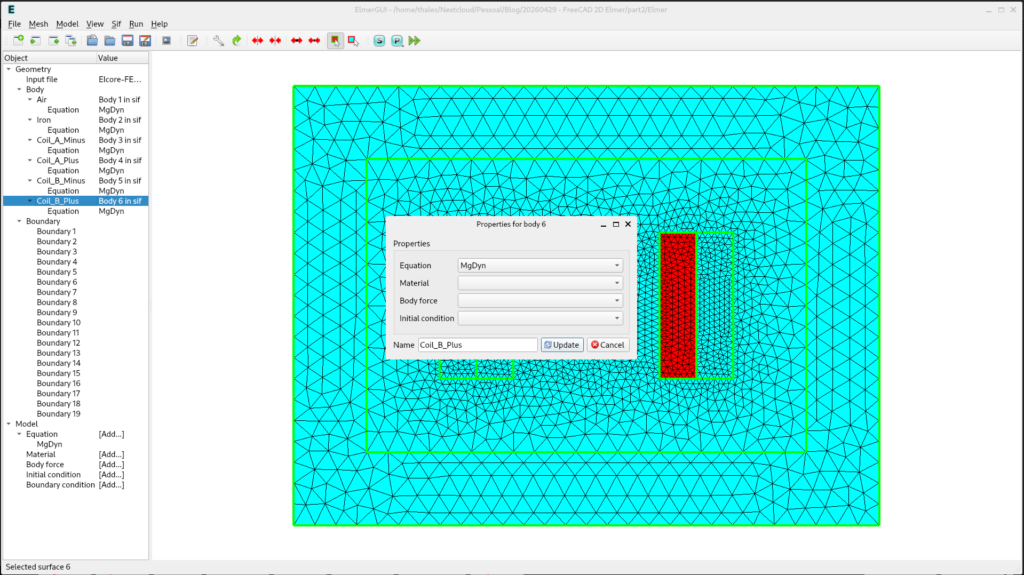
Materials and Body Identification
Before assigning materials, it is best practice to rename your bodies for better organization. Double-click the numbered bodies in the left menu to rename them (e.g., Core, Coil_A, Air).
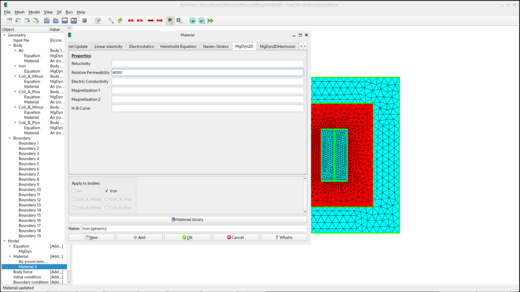
Now, apply the materials via Model >> Material >> Add:
- Air and Coils: Choose “Air” from the Material library and apply it to the Air and Coil bodies.
- Core (Iron): Select “Iron”. In the MgDyn2D tab, set the Relative Permeability to 4000.Now we can go to Material and click in [Add..]. Click in the Material library. Chose Air and Apply to bodies Air and Coils. Follow the same process, but now, select the Iron material.
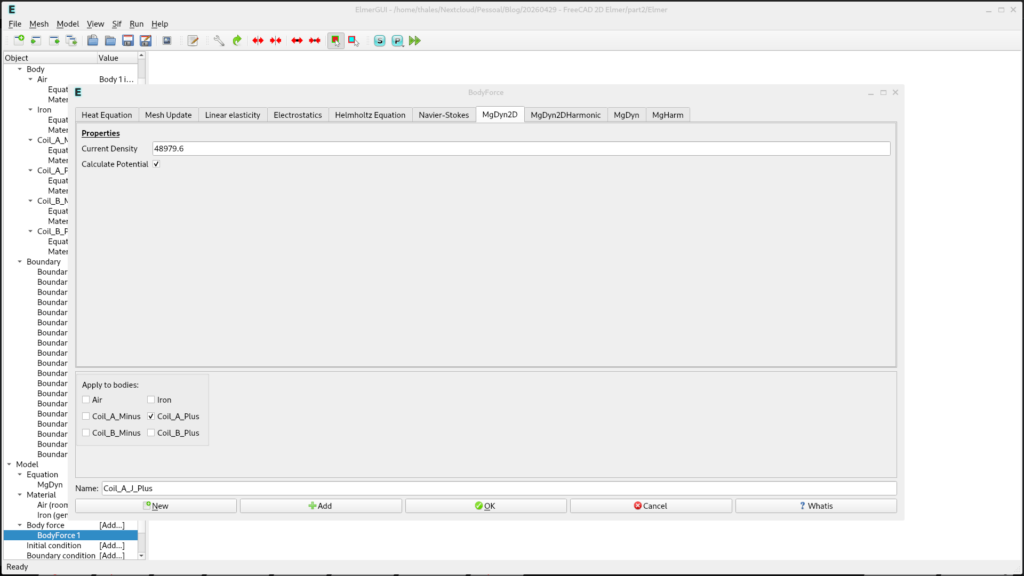
Body Force: Adding the Current Source
We must add the current source for the primary winding. In ElmerGUI, we enter the total surface current density (J). If we consider a total current of 60\ A.e, the surface current density is calculated as:
- Go to Model >> Body Force >> Add.
- In the MgDyn2D tab, check Calculate Potential and enter the calculated value above.
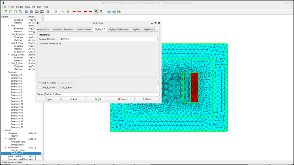
- Create a second Body Force for the opposite coil using a negative value to represent the return path of the current.
Create a new Body force, but now you should choose the opposite coil and put a negative surface current value.
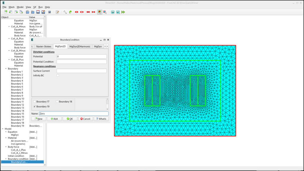
Boundary Conditions
Finally, we define the simulation boundary.
- Go to Model >> Boundary Condition >> Add.
- Select the outer boundary of the air domain.
- Set the Dirichlet Potential to 0. This ensures the magnetic flux is contained within our simulation space.
The Sif File and Running the Simulation
We are now ready for the first simulation run.
- Click on Sif in the upper bar menu and select Generate.
- Click Sif again and select Edit. You will be able to read every modification we’ve made in text format.
- After checking the settings, click the Run icon to start the solver.
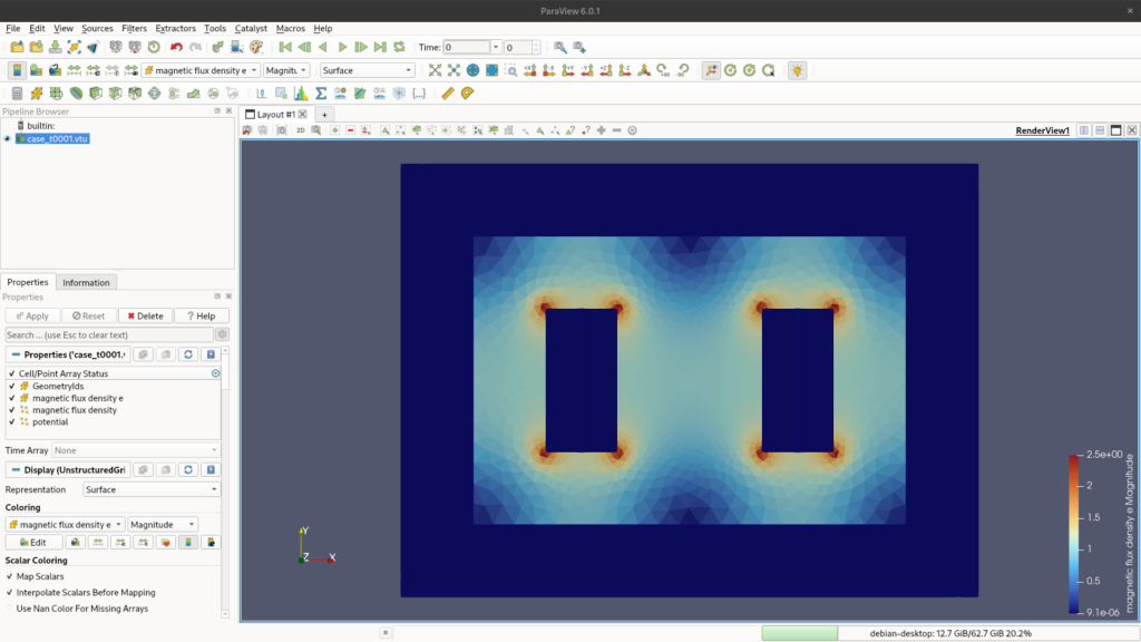
Paraview Results
If everything went fine, the solver will finish, and you will be able to view the results in Paraview. We will discuss the visualization of flux lines and density in our next topic!